WORKING PAPER

Volume Delay Function Validation

Travel models attempt to iteratively predict the demand for automobile travel and the resulting travel speed on roadway segments. The estimation of travel demand is complex and, for MTC, described in detail here. The estimation of travel speed is fairly straightforward and uses so-called “volume delay functions”, which estimate congested travel speed as a function of each roadway’s demand, free-flow speed, and effective capacity. During MTC’s Travel Model One development efforts, our legacy volume delay functions were retained.

The purpose of this memorandum is to investigate the reasonableness of the input assumptions which inform the volume delay functions as well as the shape of the volume delay curves themselves. Data from the Caltrans Performance Measurement System (PeMS) database is used in the analysis.

Travel model validation efforts often focus on comparing observed and estimated traffic volumes and point-to-point average speeds. MTC’s model validation efforts focus, instead, on observed and estimated traffic volumes and, the subject of this memorandum, the underlying assumptions that inform our volume delay functions. By so doing, we ask: if the demand is correct, are the models capable of reliably predicting travel speed? This approach should facilitate a more robust examination of our model system’s ability to replicate travel speed than point-to-point average speed comparisons, which are confounded by differences in estimated and observed traffic flow.

Background

MTC’s Travel Model One uses a typical aggregate static user equilibrium assignment method to predict the routing of vehicles. This approach, which is nearly ubiquitous across regional modeling practice in the United States, makes several important assumptions, as follows:

• Demand on a roadway segment during a finite time interval can exceed the segment’s supply/effective capacity. For example, if 4,000 vehicles want to traverse a section of roadway during a period of time in which the road can handle no more than 3,000 vehicles, the model responds by predicting travel through the corridor will be very slow, but still possible.
• The delay resulting from high demand on a roadway segment is contained entirely within that segment (i.e., queues do not form at bottlenecks and cause upstream delay; rather, the bottleneck is contained on the segment of roadway where the bottleneck occurs).
• An equilibrium condition is found such that no vehicles moving betveen any single origin/destination pair can achieve a substantially faster travel time by switching routes.

In the Travel Model One application, the demand and resulting congested conditions are described separately for five time periods which, when combined, encompass an entire typical weekday, as follows:

• early morning, 3 am to 6 am;
• morning commute, 6 am to 10 am;
• midday, 10 am to 3 pm;
• evening commute, 3 pm to 7 pm;
• evening, 7 pm to 3 am.

In aggregating travel into these time periods, we are explicitly assuming that congestion is constant within each time period. We know this is not true, e.g., traffic is almost always heavier from 7 to 8 am than from 9 to 10 am. However, we make this, and numerous other simplifications, to increase the computational efficiency and tractability of the model system.

To predict congested speeds on freeways, MTC uses so-called “BPR Curves”, the form originally developed by the Bureau of Public Roads. The shape of the curves are discussed in more detail in a later section of this document.

The Caltrans PeMS database compiles roadway monitoring data collected continuously via loop detectors to support traveler information systems. Historical data can be downloaded from the PeMS website. Records for every five- or sixty-minute interval are available. The data includes observed flow, sensor occupancy, and speed for each working detector across the State.

PeMS Data Preparation

The MTC travel model predicts traveler behavior for a typical weekday – when school is in session, the weather is clear, no major accidents occur on the roadway, etc. To extract data that best represents this abstract concept, the following process was used to filter the PeMS data:

• Begin with the hourly data, which includes estimates af average flow, sensor occupancy, and speed for every hour in the subject day.
• Only consider data from the following months: March, April, May, September, October, and November.
• Only consider data from the following days of the week: Tuesday, Wednesday, and Thursday.
• Consider data from every past full historical year for which data is available. At the time of writing, this includes 2005 through 2015.
• Only consider data from functioning detectors. More precisely: records for which 100 percent of the observations that make up the computed averages is observed, rather than imputed (Caltrans imputes data when the detectors are down or working intermittently).

One more step is carried out in a separate script to prepare the PeMS data for this analysis specifically (the data resulting from the above steps is used for a variety of purposes):

• Only consider sensors on the following routes: 4, 17, 24, 80, 84, 85, 87, 92, 101, 237, 280, 380, 580, 680, 780, 880, and 980. While MTC mapped many of the PeMS sensors to our travel model network, we did not map them all. As such, we cannot ensure that each sensor is mapped to a roadway of a known – to the travel model – facility type. To increase the chances that every sensor we are examining is on a facility designated as a “freeway” in our travel model, we first exclude any sensors that are mapped to non-freeways and then only select routes that are, in the Bay Area, largely grade-separated freeways.

After extracting hourly data, for each year of typical weekdays, we compute the following statistics:

• median, average, and standard deviation of flow (vehicles passing the sensor);
• median, average, and standard deviation of vehicle speed; and,
• median, average, and standard deviation of sensor occupance (the share of time a vehicle is above the sensor).

Do further cull problematic data, we eliminate sensor/hourly records with fewer than fifteen observations. We then eliminate observations from sensors with a maximum hourly flow of 150 vehicles or more that record a flow of zero; the idea being that if a sensor records zero vehicles during an hour in which more than 150 vehicles have been observed, it’s more likely that the sensor is broken or the lane/roadway closed than it is that the observation (of no vehicles) is correct.

We then compute a flow-weighted speed and occupancy estimate for each of the time periods in Travel Model One for each observation day for each sensor. We then compute the median, average, and standard deviation of these estimates across all typical weekdays in a calendar year. The details of these procedures can be reviewed in the implementation script.

Roadway Capacity

Travel Model One uses a simple look-up table to estimate each roadway’s effective operating capacity. Specifically, a roadway’s facility type and area type determine the roadway’s capacity. A facility’s area type is determined by the use of land immediately adjacent to the roadway using an area type density measure, which is computed as follows:

area type density index = (total population + 2.5 * total employment)/(residential acres + commercial acres + industrial acres)

Each link is assigned one of six area type categories, as shown in Table 1. The thresholds are not strict and are hand-smoothed to make them continuous across the network. Importantly, in this document we are only examining the capacity of “freeways”, which is one of ten facility types used in Travel Model One (each of the ten have similar capacity assumptions). As noted above, most all of the PeMS sensors are on roadways the travel model designates as “freeways” and we took the above-noted steps to filter out routes that we would not expect to be designated as freeways.

The capacities assumed for freeways in each of the six area types are also shown in Table 1. We know that freeways do not behave in as uniform manner as the table implies: each segment, even adjacent segments in the same urban environment, likely has a slightly different effective capacity due to differences in lane widths, shoulder widths, horizontal alignment, vertical alignment, pavement condition, presence of combination trucks, adjacent visual distractions, presence of weaving sections, etc.

Table 1

Assumed Capacity Estimates by Area Type

Area Type	Area Type Density Index (from, to)	Assumed Freeway Capacity (passengers cars per hour per lane)
Regional core	300, infinity	2050
Central business district	100, 300	2050
Urban business	55, 100	2100
Urban	30, 55	2100
Suburban	6, 30	2150
Rural	0, 6	2150

Now that we’ve detailed our observed data and outlined the assumptions behind Travel Model One’s input capacity assumptions, we can begin our first line of inquiry. We start with a basic question: do the PeMS data support segmenting freeway capacity by Travel Model One’s area type index categories? And, if so, our are assumed capacities correct?

We answer this question via the following steps:

1. Identify the area type for each PeMS station. This is done by simply locating the nearest travel analysis zone to the station; the resulting map is shown in Figure 1.

2. Compute the roadway density in vehicles per mile per lane by taking the ratio of the observed flow (in vehicles per hour per lane) and the observed speed (miles per hour).

3. Plot the observed flow by the observed density for the one-hour time periods during which we are most likely to observe the maximum flow. Figure 2 shows the familiar (to traffic engineers) flow/density relationship for four hours during the morning commute. Figure 3 shows the flow/density relationship for four hours during the evening commute.

4. Using Figure 2 and Figure 3, determine the one-hour time period during which flow is highest. For this time period, plot the flow/density relationship by area type. This is done in Figure 4 for the highest-flow morning commute hour and in Figure 5 for the highest-flow evening commute hour.

5. Compute maximum flow, and other metrics to frame the maximum, statistics by area type. These results are shown in Figure 6 for the morning commute hour and Figure 7 for the evening commute hour.

Figure 1

Location and Area Type of PeMS Stations

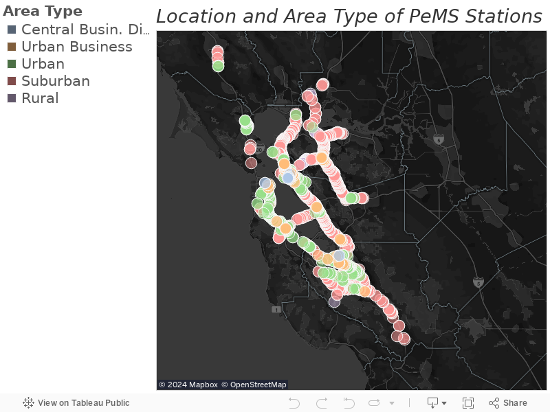
Figure 2

Flow versus Density Across All Stations during the Morning Commute

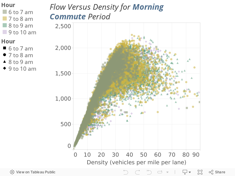
Figure 3

Flow versus Density Across All Stations during the Evening Commute

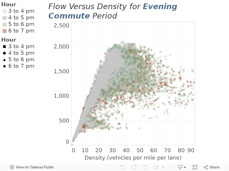
Figure 4

Flow versus Density by Area Type during the Morning Commute

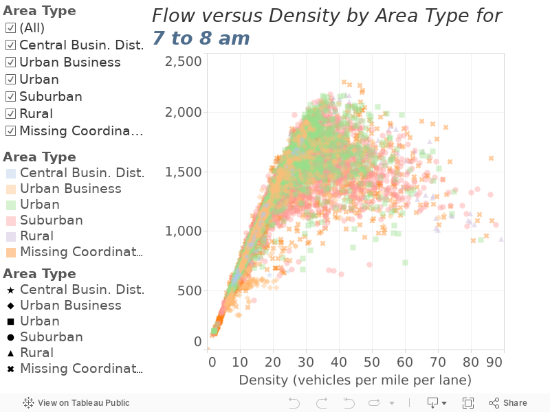
Figure 5

Flow versus Density by Area Type during the Evening Commute

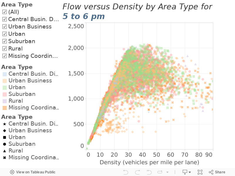
Figure 6

Implied Capacity Estimates by Area Type during the Morning Commute

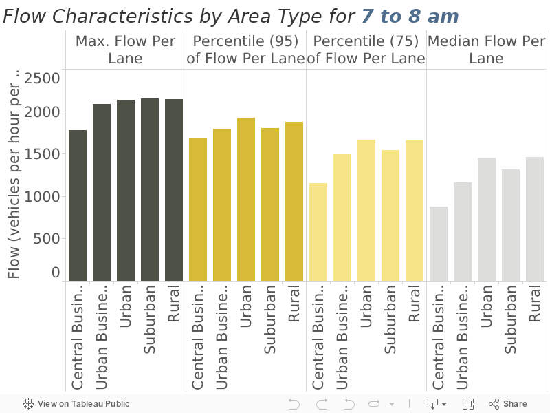
Figure 7

Implied Capacity Estimates by Area Type during the Evening Commute

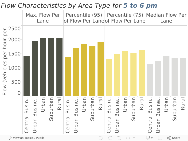
The results of the above steps are shown in Table 2. At first glance these numbers appear to support MTC’s approach of segmenting capacity by area type as well as the range of our capacity assumptions. One exception is the low capacity estimates for the “central business district” area type, for which our maximum observed flows (1780 and 1420) are quite a bit lower than our assumption of 2050 vehicles per hour per lane. Unfortunately, we have many fewer stations and observations for the central business district (only 11 in the dataset) than we do the other area types. However, the results do suggest a reduction in the capacity of freeways in this area type is warranted.

The other exception is the seemingly more efficient use of roadways during the morning commute relative to the evening commute. As travelers departure times are more consistent in the morning, there seems to be decent theoretical and, per Table 2, empirical, motivation for higher capacity assumptions in the morning commute period relative to the afternoon.

Table 2

Implied Capacity Estimates by Area Type

Area Type	Implied Capacity during Morning Commute	Implied Capacity during Evening Commute
Regional core	Insufficient data	Insufficient data
Central business district	1780	1420
Urban business	2090	1950
Urban	2140	2060
Suburban	2150	2060
Rural	2150	2040

Free-flow Speed

Travel Model One uses a simple look up table to determine the free-flow speed (i.e., the speed at which vehicles travel when there is no congestion) on each roadway segment. Similar to the capacity assumption, the free-flow speed is determined by two variables: facility type and area type. For freeways (again, one of ten facility types used by Travel Model One), the assumed free-flow speeds are shown in Table 3.

Table 3

Assumed Free-flow Speed Estimates by Area Type

Area Type	Assumed Speed (miles per hour)
Regional core	55
Central business district	55
Urban business	60
Urban	60
Suburban	65
Rural	65

Using the PeMS data, we can ask two interesting questions: (i) is it reasonable to segment free-flow speed by MTC’s area types and (ii) are the free-flow speed assumptions reasonable. As with the previous discussion on capacity, it is important to note that we are only examining the assumptions made for freeways.

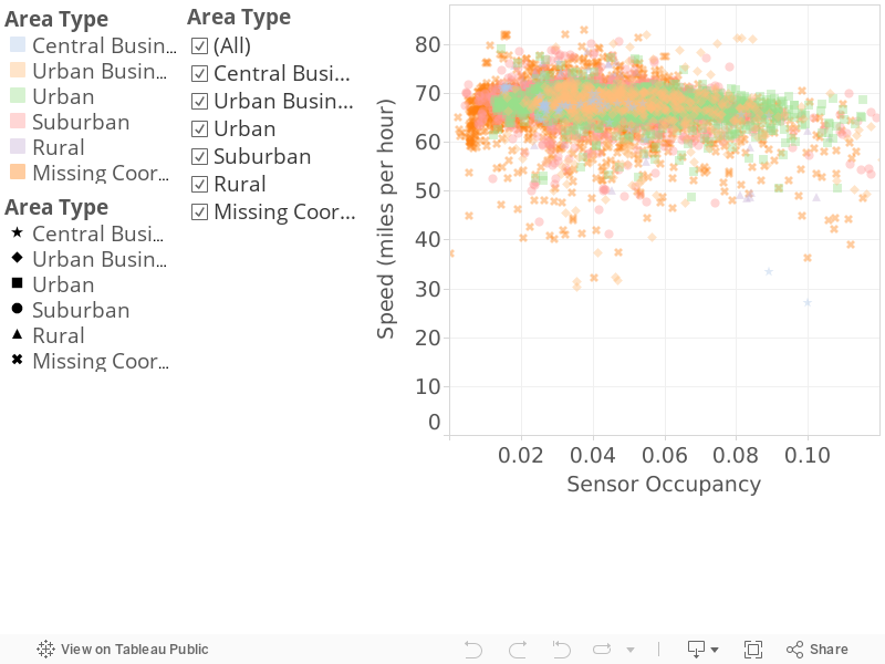
To estimate the free-flow speed of the Bay Area residents we are simulating in our travel model, we select the time periods at the beginning of the morning commute and the end of the evening commute, as these times likely include resident travelers and have little congestion. Figure 8 plots the observed speed of travelers during the hour from four to five a.m. against sensor occupancy (i.e., the percentage of time the loop detector has a vehicle above it), segmented by area type. A companion plot is presented in Figure 9 for the hour from seven to eight p.m. The vast majority of observations in these plots occur at very low sensor occupancy rates, suggesting – as hoped – little congestion.

Figure 8

Observed Speed by Area Type from 4 to 5 am

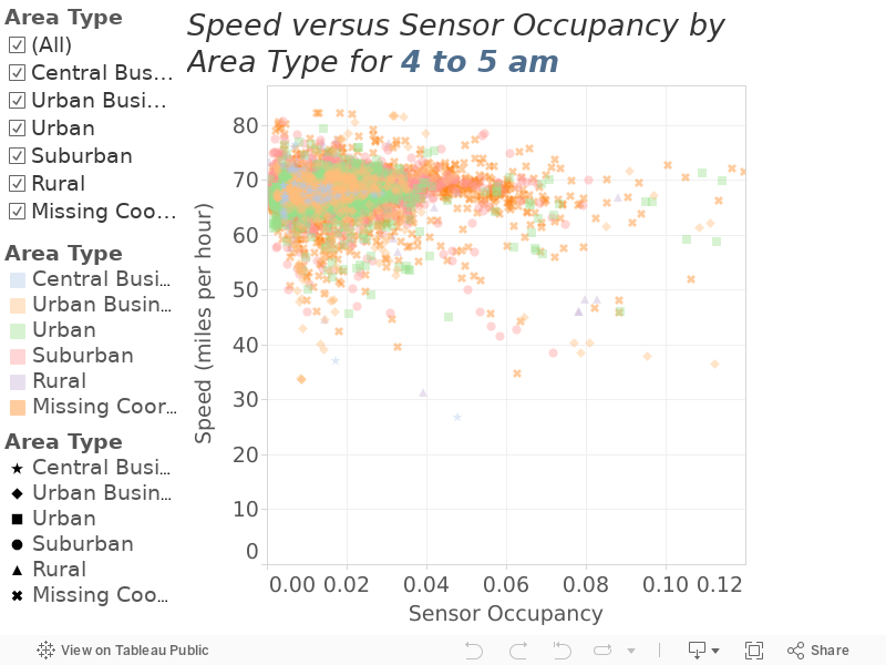
Figure 9

Observed Speed by Area Type from 7 to 8 pm

Speed statistics are extracted from the data and shown in Figure 10 and Figure 11. Table 4 below summarizes the median speeds from the two charts and presents those as the implied free-flow speeds. Note that in the case of trying to estimate the physical capacity, using the maximum makes the sense as we are trying to gauge how many cars can physically move through the roadway segment. In the case of free-flow speed, we are trying to understand the typical behavior of the typical driver, which logically points to using the median.

Figure 10

Speed Characteristics by Area Type (4 to 5 am)

Figure 11

Speed Characteristics by Area Type (7 to 8 pm)

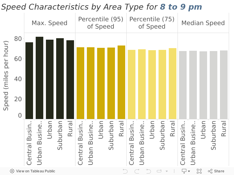
Table 3

Implied Free-flow Speed Estimates by Area Type

Area Type	Implied Free-flow speed during Morning Commute	Implied Free-flow Speed during Evening Commute
Regional core	Insufficient data	Insufficient data
Central business district	67.7	67.6
Urban business	67.9	67.9
Urban	67.2	67.3
Suburban	67.3	67.6
Rural	67.9	68.2

The evidence in Table 3 suggests that segmenting free-flow speed by area type is not warranted. Two potentially superior approaches may be: (i) using 67 miles per hour for all freeways or (ii) using the posted speed limit. The latter suggestion may be feasible in MTC’s forthcoming Travel Model Two, which uses a navigation network for which posted speeds are available.

Volume Delay Functions

Travel Model One uses a variation of the Bureau of Public Road (BPR) curve to compute congestion on freeways. We refer to these curves as “volume-delay functions”. The function is as follows:

congested travel time = free-flow travel time * (1 + alpha * (4/3 * volume/capacity)^beta),

where, in Travel Model One, alpha is 0.20 and beta is 6.0.

To use the BPR curve, we must provide (a) a free-flow speed on each roadway segment; (b) an estimate of effective capacity for each roadway segment; and, (c) determine the parameters alpha and beta. The previous two sections of this document discussed the assumptions we make regarding (a) and (b) and used the PeMS data to assess the reasonableness of those assumptions. Comfortable that our assumptions for free-flow speed and capacity are, while not perfect, reasonable, we can use the estimates of observed flow from the PeMS database as a surrogate for demand and then compute estmates of congested travel time using the BPR curve. The estimated travel time can be converted to speed and compared directly to the observed speeds in the PeMS database. This examination should help us assess the reasonableness of the BPR curves.

The PeMS database contains estimates of traffic flow (i.e., the number of cars that pass a roadway detector per unit of time). Flow is a revealed expression of an unobserved demand for vehicle travel (i.e., the number of cars that want to pass a roadway detector per unit of time). Travel Model One estimates demand. The flow on a roadway segment cannot exceed a roadway’s effective capacity; the demand can. When examining the PeMS data, we will often observe similar observed flows for roadways operating at very different speeds: low flow when traffic is light and speeds are high and similarly low flow when traffic is heavy and speeds are low.

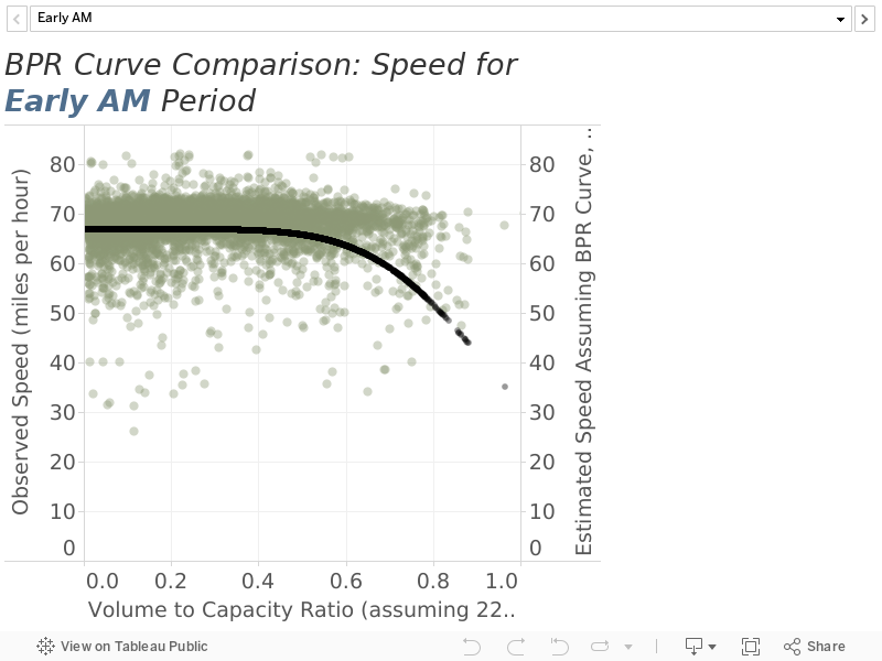
The first assessment of the performance of the volume-delay functions plots the observed volume-to-capacity ratio against observed travel speed along with the assumed BPR curves. We use “volume” here to represent either observed flow (when plotting the PeMS data) or unobserved demand (when plotting the BPR curves). These charts are shown in Figure 12 and are segmented by time period. Important notes regarding these plots are as follows:

• We assume a capacity of 2,200 vehicles per hour per lane and a free-flow speed of 67 miles per hour for each of the stations.
• We include points for which the demand exceeds the roadway capacity. In the PeMS data, flow is low, so these points appear close to the origin on the chart (low observed speed, low volume-to-capacity ratio). If we knew the demand, however, these points would appear in the lower right-hand corner of the plot (low observed speed, high demand-to-capacity ratio). We include these points in the chart, but note that “volume” for the PeMS data has a different meaning than “volume” for the BPR curves.
• The plots generally show the curves fit the data reasonable well.

Figure 12

Observed/Estimated Speed against Observed Volume-to-Capacity Ratio by Time Period

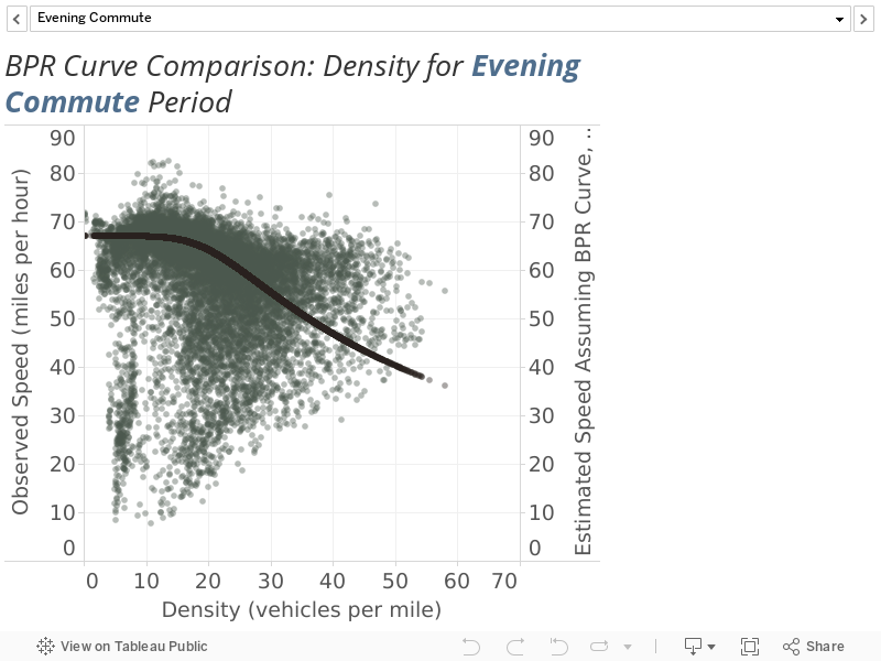
The second assessment of the performance of the volume-delay functions focuses on the aforementioned problematic cases in which demand exceeds capacity. Here, density, which is the quantity hourly flow divided by speed, is plotted against speed. These plots reveal observed travel speeds when densities exceed the critical threshold at which speeds begin to degrade (which is around 30 vehicles per mile, as shown in Figure 2 and Figure 3). Figure 13 compares the BPR curves to the observed data by time period. These charts again assume a capacity for each station of 2,200 vehicles per hour per lane.

Each of the commute period plots show the curves perform okay at high densities.

Figure 13

Observed/Estimated Speed against Density by Time Period

Conclusion

In sum, this investigation demonstrates that MTC’s Travel Model One deploys reasonable procedures for translating vehicle demand to roadway speeds. Improvements to these procedures will be explored during the Travel Model Two development effort, details of which are available here.